Deriving the Acoustic Wave Equation

Jonathan South Fundamentals August 19, 2018

FOREWORD

While this is a derivation involving somewhat involved maths and physical concepts, I have purposefully made it quite “verbose” and explanatory in nature. Hopefully (if you are at least at the undergraduate physics level), there should not be too many stumbling points and should make logical progression without large leaps of faith. As such, I wouldn’t call it a compact derivation or post.

Why Waves?

We are so used to describing sounds as “waves”, or referring to implied realisations of sound as a wave (frequency/amplitude/phase), the actual physics is sometimes overlooked or forgotten. The question “why waves?” can be answered (either completely, or completely unsatisfying-ly) by “it satisfies the wave equation”. Starting from a few simple assumptions, we’ll build a mathematical description of the way sound propagates, which you will hopefully recognise as a wave equation. To cover the most interesting and applicable cases, we’ll concentrate on sound propagating in gaseous mediums (sorry hydro-acoustics).

Properties of the Medium

Conceptually, gases are a collection of atoms/molecules which travel quite fast, bouncing off each other and boundaries. We may have some expectation for information (sound/disturbances) to be able to “travel” through the gas as particles bounce off one another, but may not be sure of the exact form which information travels. To build the technical understanding, we need to need to be comfortable with describing some macro properties of the gas, particularly pressure $\left(P\right)$ and density $\left(\rho\right)$ .

We can pose some base assumptions, without too much in depth consideration

Gas particles move, and as they do the density of the gas changes (more particles in a given volume gives a higher density and vice versa),
Pressure changes with some relation to this density change (higher density, more particle collisions, higher pressure, and vice versa),
Pressure gradients cause gas particles to move (particles tend to move from regions of higher pressure to lower pressure).

From these assumptions, we can see that for a given disturbance there is already a cyclic cause and effect emerging. Assumption 1, leads to 2, leads to 3, leads back to 1 and so on.

Equilibrium

Starting with an “undisturbed” gas, seems a bit of a problem, as the particles are naturally moving, colliding and interacting with seemingly random conditions all the time. We can however talk about a gas in a state of equilibrium, where pressure and density are consistent throughout the medium. From here, we can also define the acoustic pressure as the “excess” pressure above equilibrium, and similarly for density:

$P = P_0 + P_{acoustic} \\ \text{where } P, P_0 \text{ are the total and equilibrium pressure respectively.}$

$\rho = \rho_0 + \rho_{acoustic} \\ \text{where } \rho, \rho_0 \text{ are the total and equilibrium density respectively.}$

Another condition falls out of this; since total pressure cannot be negative, $P_{acoustic} \leq P_0$ .

Pressure and Density

In Assumption 2, we posited that pressure changes “in some relation” to density. Lets formalise this using some function, $f\left(\rho\right)$ . The next step of linearisation is very common in physics problems when you either have a very complicated relationship between variables, or are just not too sure of what the relationship is. We use the Taylor expansion of $f$ , but then say we only want linear terms and lower, we get a relatively simple functional relationship between variables albeit with a pretty big caveat.

The linearisation only holds for small deviations around the expansion point.

Taking the expansion around the equilibrium density yields

$\begin{aligned}P=& f\left(\rho\right) \\ =& f\left(\rho_0\right) + f^\prime \left(\rho_0\right) \left(\rho-\rho_0\right) \\ =&P_0 + f^\prime \left(\rho_0\right) \rho_{acoustic}\\=&P_0 + \kappa \rho_{acoustic} \ \ \ \ \ \ \mathbf{\left(II\right)}\end{aligned}$

Where $f(\rho_0) = P_0$ , which hopefully makes sense, and we’ve set $f^\prime\left(\rho_0\right) = \frac{d P}{d \rho}\vert_{\rho_0} =\kappa$ . Moving forward, we must remember that by linearising the equation we should only consider small deviations in density around the equilibrium point.

Displacement and Density

To formalise Assumption 1, consider the displacement of gas at a time and location in space $\chi \left(x , t \right)$ . This function describes the displacement of gas particles (in the $x$ direction) in a region from their average equilibrium position, in response to a movement of gas around it.

For a visual reference, Figure 1 shows a collection of gas particles at equilibrium (1,2), and when disturbed by a sound wave arriving from the left (3,4).

At equilibrium, the gas particles at $\left(x, t \right)$ , are just found at $x$ . Particles just next door, at $\left(x+\Delta x, t \right)$ are similarly located at $x +\Delta x$ . The volume (for some perpendicular area $A$ and mass $m$ of gas in this little snapshot of equilibrium is thus

$\begin{aligned}V_0=& A \left[ \left( x +\Delta x\right) - x \right] \\ =& A \Delta x \\ \implies m_0 =& \rho_0 A \Delta x \end{aligned}$ .

When disturbed by movement, the particles at $\left(x, t \right)$ are found at $x + \chi \left( x_a, t \right)$ , and the particles at $\left(x +\Delta x, t \right)$ are found at $x+\Delta x + \chi \left(x +\Delta x , t \right)$ . The volume (for the same $A$ ) and mass of gas in the snapshot of disturbed gas is

$\begin{aligned}V=& A\left[ \left(x +\Delta x + \chi \left(x +\Delta x \right)\right) - \left(x + \chi \left( x, t \right)\right)\right] \\ =& A\left[ \Delta x + \chi \left(x +\Delta x \right) - \chi \left( x, t \right)\right] \\ \implies m =& \rho A \left[\Delta x + \chi \left(x +\Delta x \right) - \chi \left( x, t \right)\right] \end{aligned}$

Now, we can argue the mass of gas (or number of particles) must not change (notice between Figure 1 (1,2) and (3,4) the number of particles in the volume does not change), thus $m_0 =m$ , giving

$\begin{aligned} m_0 =& m \\ \rho_0 A \Delta x =& \rho A \left[\Delta x + \chi \left(x +\Delta x \right) - \chi \left( x, t \right)\right] \\ \rho_0 \Delta x=&\rho \left[\Delta x + \frac{\partial \chi }{\partial x}\Delta x\right] \\ \rho_0 =& \rho \left[1 + \frac{\partial \chi }{\partial x}\right] \\=& \left(\rho_0 + \rho_{acoustic}\right) \left[1 + \frac{\partial \chi }{\partial x}\right]\\=& \left(\rho_0 + \rho_{acoustic}\right) \frac{\partial \chi }{\partial x} +\rho_0 + \rho_{acoustic} \\ \implies \rho_{acoustic} =&-\rho_0 \frac{\partial \chi }{\partial x} - \rho_{acoustic} \frac{\partial \chi }{\partial x} \\ =& -\rho_0 \frac{\partial \chi }{\partial x}\ \ \ \ \ \mathbf{\left(I\right)}\end{aligned}$ .

We’ve used a slightly altered approximation for the partial derivative of $\chi$ to move from the first to the second line. The approximation in the last line is valid as we know $\rho_{acoustic} \ll \rho_0$ .

Figure 1 – Gas particles at equilibrium and when disturbed.

Figure 1 – (1,2) Particles at their equilibrium position. (3,4) Particles moved by an incoming sound in the positive x direction.

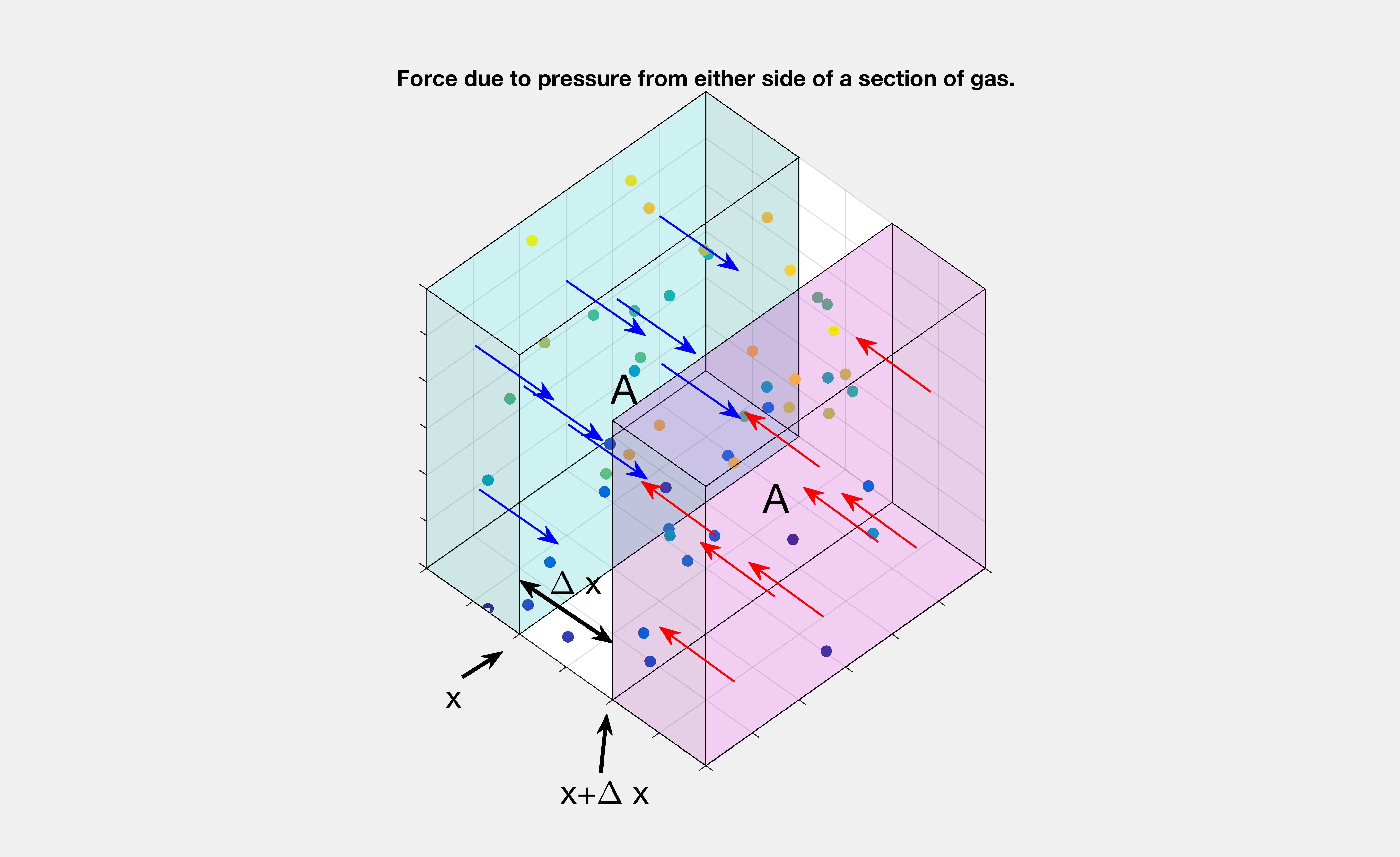
Displacement and Pressure

Working now with Assumption 3, and taking a similar approach to the previous section. A thin section of air at equilibrium has mass $m_0 = \rho_0 A \Delta x$ . Newtons second law gives us a relationship between the force acting on this section of gas, and the acceleration it undergoes. We already have $\chi$ describing the displacement, so the second partial derivative with respect to time gives us the acceleration at a point.

$\begin{aligned} \Sigma F\left(x,t\right) = \rho_0 A \Delta x \frac{\partial^2 \chi}{\partial t^2} \end{aligned}$

To find the forces acting on this section of gas, consider the pressures (force per unit area) at the “left” side , which would be given by $P\left(x,t\right) A$ . This is the force due to pressure from gas in the cyan region of Figure 2. The force on the “right” side would be $-P\left(x+\Delta x\right) A$ , from pressure of the gas in the magenta region of Figure 2.

So the total force on the section is

$\begin{aligned} \Sigma F\left(x,t\right) = P\left(x,t\right)A -P\left(x+\Delta x\right) A =& - A \frac{\partial P}{\partial x} \Delta x \end{aligned}$

where the partial derivative is found using the same approximation as in the last section.

Putting this with the previous equation we have

$\begin{aligned} -A \frac{\partial P}{\partial x} \Delta x &= \rho_0 A \Delta x \frac{\partial^2 \chi}{\partial t^2} \\ -\frac{\partial P}{\partial x} &= \rho_0 \frac{\partial^2 \chi}{\partial t^2}\\ -\frac{\partial P_{acoustic}}{\partial x} &= \rho_0 \frac{\partial^2 \chi}{\partial t^2}\ \ \ \ \mathbf{\left(III\right)}\end{aligned}$

We simplified the partial derivative of $P$ as we know $P_{acoustic}$ is the component that changes.

Figure 2 – Force and Pressure on a Section of Gas.

Figure 2 – Force due to pressure from either side of a section of gas.

Putting it all Together

With the mathematically formalised versions of our 3 assumptions, we can combine them and eliminate some variables.

First, using $\begin{aligned}\mathbf{\left(II\right)}\end{aligned}$ and taking the partial with respect to $x$ gives

$\begin{aligned} P=&P_0 + \kappa \rho_{acoustic}\\ \frac{\partial P}{\partial x} =&\kappa \frac{\partial \rho_{acoustic}}{\partial x}\\ \frac{\partial P_{acoustic}}{\partial x} =&\kappa \frac{\partial \rho_{acoustic}}{\partial x}\end{aligned}$

Substituting into $\begin{aligned}\mathbf{\left(III\right)}\end{aligned}$ gives

$\begin{aligned} -\kappa \frac{\partial \rho_{acoustic}}{\partial x} &= \rho_0 \frac{\partial^2 \chi}{\partial t^2}\end{aligned}$

Similarly taking the partial derivative of $\begin{aligned}\mathbf{\left(I\right)}\end{aligned}$ with respect to $x$ and substituting into above, gives

$\begin{aligned} \rho_{acoustic} =& -\rho_0 \frac{\partial \chi }{\partial x} \\ \frac{\partial \rho_{acoustic}}{\partial x} =& - \rho_0 \frac{\partial ^2 \chi}{\partial x^2} \\ \\ \implies \kappa \rho_0 \frac{\partial ^2 \chi}{\partial x^2} =& \rho_0 \frac{\partial^2 \chi}{\partial t^2} \\ \kappa \frac{\partial ^2 \chi}{\partial x^2} =& \frac{\partial^2 \chi}{\partial t^2} \\ \frac{\partial ^2 \chi}{\partial x^2} = & \frac{1}{c^2}\frac{\partial^2 \chi}{\partial t^2}\end{aligned}$

Which is (finally) our beloved wave equation for particle displacement, with the speed of the wave $c = \sqrt{\kappa } = \sqrt { \frac{d P}{d \rho}\vert_{\rho_0}}$ .

Summary

There is unfortunately a lot that we’ll leave at face value here (What makes this a wave equation equation? What about pressure? What about sound in three dimensions?), but that’s probably enough for this post. The main goal of introducing this derivation is to:

Show how the formalisation a few simple physical assumptions can lead to a useful result,
Show that sound will indeed propagate as waves,
Introduce the wave equation.

The wave equation is so important because it is an exact mathematical description of how sound propagates and evolves. Any situation could be modelled using this. Sound indoors, outdoors, barriers, absorption, diffusion, reflections, transmissions, high frequency, low frequency. It’s all covered. But, PDE’s are messy and hard. They have analytical solutions in only the simplest of cases, and computational models have their own limitations. Hence we introduce other potential solution methods such as ray acoustics, source/propagation simplifications, spectral and pseudo-spectral models, empirical models and even physical scale models to assist in solving specific problems.

References

This derivation follows the methods used by Feynman, found here. Feynman’s methodology is wonderfully conceptual and is build from minimal assumptions. There are many alternate approaches (such as starting with the ideal gas law).

All figures are original.

Tags: acoustics, derivation, maths, physics, sound