Auralising the “Tongue Drum”

Previously, we used finite element analysis to visualise the modal patterns and frequencies of the simple percussive instrument, the “Tongue Drum”. For this analysis, we’re going to switch from the frequency domain, to the time domain, with the ultimate goal of “hearing” our fully simulated drum!

We’re back in MATLAB’s pde toolbox, this time leveraging some some inclusions in the 2019a release – formulating the pde model as a transient-solid. The general procedure start the same as the modal analysis; import geometry and then create the mesh. From here, we then specify boundary conditions, as well as the initial loading/forcing which drives the transient response. To save on computation time, I’m also feeding the solver the modal results, which uses the modal superposition method to calculate the transient solution (this is orders of magnitude faster, but not quite as accurate. Since I’m calculating such a long solution in the time domain, its a no brainer to use this method).,

Striking the Drum

In real life, we strike the drum with a physical object to drive a transient response from the solid. In the model, we simulate this strike with a pressure/force load over a specified period of time. I ended up with some less than ideal implementations mostly due to the faceting of the .stlgeometry imported in to MATLAB, settling on the following 3 “strikes”.

1. A very short downwards force on the 4 vertices on the tip of the larger tongue. Aiming to “play” the lower note.
2. A very short downwards force on the 4 vertices on the tip of the smaller tongue. Aiming to “play” the higher note.
3. A very short inwards pressure across the entire main face (top, note tongues and sides) of the drum. Not very physical, but should be interesting.

Extracting a Time Signal

The solver returns the displacement of each of the mesh nodes for each time step, which we need to manipulate to get our time signal. It’s no good just looking at one mesh point – it may not vibrate in a way that is representative of the entire solid, and we want to capture the sound of the whole drum. For a quick and dirty method, I implemented a simple propagation model. It assumes that each mesh node radiates as a point source, directly to a point where we want to “listen” to the drum. The signal from each mesh node is appropriately delayed and attenuated with the superposition of each taken as the resulting signal. Not super sophisticated, but it does get the job done.

Results

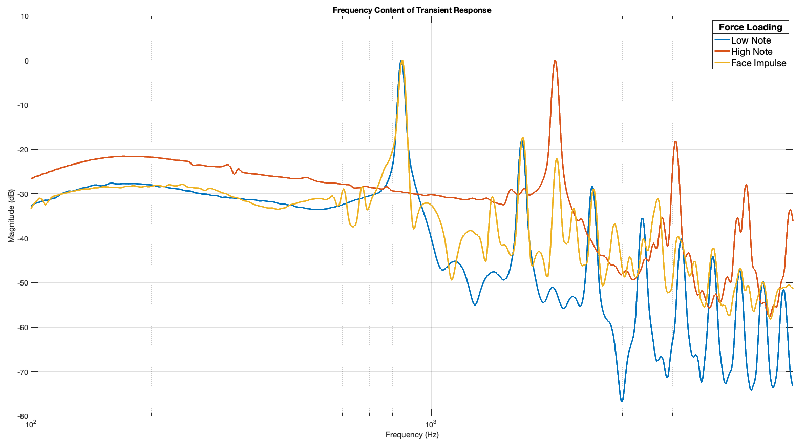
And here are the time signals for your listening pleasure (or displeasure)! I’ve also shown the spectral content for further discussion.

We can see that the lower note has a fundamental at 850hz, with the high note sitting up at about 2kHz, with the overtone series for each note clearly visible.

The time domain signals leave a lot to be desired, but I think they are an interesting first look in to a time domain analysis. Lots more that I’d like to explore, but I think I’m going to shelve it for now and move on to some other projects!

Code

The main code for the solver. Not included is the analysis code, let me know if you are interested.

 
 
 %% Properties
  
 % 0 or 1 to plot geometry or mesh
 plotGeometry = 1;
 plotMesh = 1;
  
 % Mesh params
 hmax = 0.03;
  
 % Material
 % Approximates steel
 E = 180e9; % Modulus of elasticity in Pascals
 nu = .265; % Poisson's ratio
 rho = 8000; % Material density in kg/m^3
  
 % Solver 
 frequencyRange = 2*pi*[100, 8000]; %frequency range for the modal solution
 fs = 16000; % Sample Rate
 tFinal = 1; % Calculation time
 t = 0:1/fs:tFinal; % time vector
  
  
 %% Modal Solution
 modalModel = createpde('structural','modal-solid');
  
 % Geometry
 geom = importGeometry(modalModel, 'tongue_drum.stl');
  
 % Visualise the Geometry
 if plotGeometry
     figure
     hc = pdegplot(modalModel, 'VertexLabels','on');
     hc(1).FaceAlpha = 0.6;
 end
  
 % Set up the PDE coefficients
 structuralProperties(modalModel,'YoungsModulus',E,...
     'PoissonsRatio', nu,...
     'MassDensity', rho);
  
 % Mesh the Geometry
 msh = generateMesh(modalModel,'Hmax',hmax,'GeometricOrder','quadratic');
  
 % Visualise the mesh
 if plotMesh
     figure
     pdeplot3D(modalModel);
     title('Meshed Geometry');
 end
  
 % Boundary Conditions
 structuralBC(modalModel, 'Face', 3 ,'ZDisplacement',0) ;
  
 %% Modal Solver
 modalResults = solve(modalModel, 'FrequencyRange', frequencyRange);
  
 %% Transient
  
 solutionName = 'face'; % Creates a directory to save results to.
  
 transientModel = createpde('structural','transient-solid');
 transientModel.Geometry = geom;
 transientModel.Mesh = msh;
 structuralProperties(transientModel,'YoungsModulus',E,...
     'PoissonsRatio', nu,...
     'MassDensity', rho);
 % Set the drum "on the ground"
 % note this does not exclude it from moving in the plane.
 structuralBC(transientModel, 'Face', 3 ,'ZDisplacement',0) ;
  
  
 % Set the type and location of force loading
 % vertices for the low and high notes. (Manually inspect the geometry plot
 % to find these.
 highVerts = [6, 8, 24, 25];
 lowVerts = [14, 15, 28, 33];
  
 % Comment/uncomment one of the below, and change the target vertices.
 %structuralBoundaryLoad(transientModel, 'Vertex', lowVerts, 'Force', [0, 0, -20], 'EndTime',10/fs);
 structuralBoundaryLoad(transientModel, 'Face', 1, 'Pressure', 10E5,'EndTime',10/fs);
  
 % Start from rest.
 structuralIC(transientModel, 'Displacement', [0;0;0], 'Velocity', [0;0;0]);
  
 %% TransientSolver
  
 tic
 transientResults = solve(transientModel,t, 'ModalResults', modalResults);
 toc
  
 mkdir('.',solutionName)
 save(join([solutionName,'/results.mat']),'transientResults', '-v7.3')