Acoustic Eigenmodes and the Helmholtz Equation

Jonathan South Fundamentals August 20, 2018

You are hopefully well aware of room modes and resonances. As the bane of home recording spaces, they have the ability to wreak havoc on small, untreated rooms. Physically, they are the result of standing waves, sound reflecting between surfaces in such a way that they reinforce themselves. They are based on the geometry of the space, with physical dimensions affecting the frequencies at which standing waves occur. Simple, regular geometries can be solved analytically, with well known results for rectangular prisms, cylinders, spheres etc. More complicated geometries require other techniques.

A Specific Solution to the Wave Equation

Starting with the wave equation (derived for 1D here, we’ll use the 3D version) for pressure.

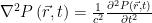
$\nabla^2 P\left(\vec{r},t\right) = \frac{1}{c^2} \frac{\partial^2 P\left(\vec{r},t\right)}{\partial t^2}$

Where of course $\nabla$ is the differential vector operator

$\nabla =\hat{i} \frac{\partial}{\partial x}+ \hat{j} \frac{\partial}{\partial y} +\hat{k} \frac{\partial}{\partial z}$

Next we take a logic leap, and say that we only want to focus on a very specific subset of solutions to the wave equation. Lets consider only situations where we

have some distribution of pressure which is static in space, but oscillates with a well defined frequency in time. Physically, these are the standing waves/room modes (standing/static in space), while mathematically we have

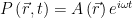
$P\left(\vec{r},t\right) = A\left(\vec{r}\right) e^{i \omega t}$

where $A \left( \vec{r} \right)$ is the spatial solution, and $e^{i \omega t}$ gives the temporal oscillations with frequency $\omega$ .

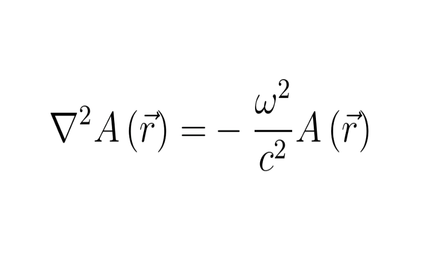
You may recognise this as essentially the “Separation of Variables” technique, commonly used in PDE analysis. Using this form of solution in the wave equation yeilds

$\begin{aligned} \nabla^2 P\left(\vec{r},t\right) =& \frac{1}{c^2} \frac{\partial^2 P\left(\vec{r},t\right)}{\partial t^2} \\ \nabla^2 \left[A\left(\vec{r}\right) e^{i \omega t}\right] =& \frac{1}{c^2} \frac{\partial^2}{\partial t^2} \left[A\left(\vec{r}\right) e^{i \omega t}\right]\\ e^{i \omega t} \nabla^2 A\left(\vec{r}\right) =& -\frac{\omega^2}{c^2} A\left(\vec{r}\right)e^{i \omega t} \\ \nabla^2 A\left(\vec{r}\right) =& -\frac{\omega^2}{c^2} A\left(\vec{r}\right) \ \ \ \ \ \ \ \ \ \ \ \ \ \ \ \ \ \mathbf{\left(I\right)}\\ 0 =& \nabla^2 A\left(\vec{r}\right)+\frac{\omega^2}{c^2} A\left(\vec{r}\right) \ \ \ \ \ \ \mathbf{\left(II\right)} \end{aligned}$

We usually set $\frac{\omega}{c}=k$ , and call $k$ the wavenumber, or the spatial frequency.

Equation $\mathbf{\left(II\right)}$ is known as the Helmholtz equation, which usually appears in that form. Looking quickly at the form of equation $\mathbf{\left(I\right)}$ , we have a vector operator that when applied (twice) to a vector function, equals a constant multiplied by that same vector function. If you were paying attention in Linear Algebra, you should recognise this as an Eigenvalue/Eigenvector problem, where $\mathbf{Mv} = \lambda \mathbf{v}$ .

This is where the slightly less common term eigenmode comes from when talking about room acoustics, or acoustics within cavities. The wave equation simplifies under separation of variables to give a function (or functions) which are solutions to the Helmholtz Equation, an eigenvalue problem.

Boundary Conditions

Now might seem like we haven’t done too much here, but at least we’ve reduced a second order PDE in time and space, to a second order PDE in space only. We don’t have enough information to solve the Helmholtz Equation until we specify the geometry of the problem, and perhaps more importantly, the boundary conditions of the geometry.

Since there is a lot to say about boundary conditions and their implementation, I’ll only touch briefly on a specific case; the perfectly reflecting boundary. Physically (but not necessarily realistically), this may be a very hard wall, which does not transmit or absorb any sound energy.

At this boundary, we don’t expect gas particles to be able to move in to the region of the wall, neither do we expect them to move away from the wall (else they should leave a perfect vacuum in their wake). This gives an immediately available boundary condition of displacement, and velocity (in the direction normal to the wall) being zero at the boundaries. However, gas pressure is what we are interested in (and one that I like to work with, given that its a scalar and more readily measured by practical equipment), so lets consider that. We know the gas displacement and velocity (again, in the direction normal to the boundary) is 0 at boundaries, and gas movement is driven by some net force acting on a small section of gas, we can reasonably say this force is 0. Since the force is proportional to the pressure differential, we then have

$\frac{\partial P}{\partial \vec{n}} = 0 \text{ where } \vec{n} \text{ is the direction normal to the boundary}$

This type of boundary condition is known as a Neumann boundary condition, in that the derivative of the function of interest is specified at the boundary.

Applications

Armed with the Helmholtz Equation and suitable boundary conditions, you can analyse a host of complicated situations. Typically, you might be asked to find resonant frequencies of certain rooms geometries, cavities or spaces, typically using numerical techniques. Some simple examples to come.

Tags: acoustics, boundary condition, cavity resonator, eigenmode, helmholtz, pde, resonance, room acoustics, room mode, standing wave

Acoustic Eigenmodes and the Helmholtz Equation

A Specific Solution to the Wave Equation

Boundary Conditions

Applications

About: Jonathan South