Simple Room Resonance Analysis

Jonathan South Modelling & Simulations, Room Acoustics September 1, 2018

Lets put some theory to the test by finding the room resonances of simple (and maybe not so simple) 2D polygonal rooms using computational methods. I’ll explain the code, and provide a file for download as well.

The Problem

To find room resonances, we need to solve the Helmholtz Eigenvalue problem (see here for why)

$\begin{aligned} \nabla^2 A\left(\vec{r}\right) =& -\frac{\omega^2}{c^2} A\left(\vec{r}\right) \end{aligned}$

We’ll limit ourselves to 2D polygonal regions, for simple geometry creation, and the fact that most rooms are uniform height (and hence the strongest axial modes are easy to calculate).

The Solution

We’ll calculate solutions using MATLAB’s PDE Toolbox, which uses finite element analysis (FEA) to solve a given PDE over the given domain. For reference, I’m using MATLAB_2016b with PDE Toolbox 2.3.

The Implementation

My hope is that the code is well commented and self-documenting (I know, you’ve been hurt before), so I’ll keep explanations minimal.

User Setup

Start with some simple user values. The polygon is defined by a 2xN array of x and y coordinates.

%% User Setup

% x/y coordinates of the room geometry. Assumed closed polygon between last
% and first coords.
polygonVertices = [[0 4 4 0];[0 0 3 3]]; %[m]

% Interval to search for resonant frequencies
fRange = [20 200]; %[Hz]

% Wave speed of the medium on the region. Approx 343 m/s for air at STP.
medium_speed = 343.0; % [m/s]

Internal Setup

The function which adds a geometry to the model pde.PDEModel.geometryFromEdges() accepts a relatively specific formulation for the geometry, which is somewhat messy to create, so I’ve abstracted that away in a helper function createRoomGeometry().

The Toolbox solves eigenvalue problems in the form of

- div(c*grad(u)) + a*u = lambda*d*u.

where u is a generic scalar field (i.e pressure) so a bit of algebra manipulates the Helmholtz equation and yields the coefficients

$\begin{aligned} u =& p \\ c =& -1 \\ a =& 0 \\ \lambda =& \omega^2 = \left(2\pi f\right)^2 \\ d =& -\frac{1}{c^2 }\end{aligned}$

Boundary conditions for a perfectly reflecting boundary are a Neumann condition, where the pressure gradient is 0 in the direction normal to the boundary. The Toolbox specifies the Neumann condition in the form of

n*(c*grad(u)) + q*u = g

corresponding to

$\begin{aligned} q =& 0 \\ g =& 0 \end{aligned}$

%% Model Setup
disp('Setting up model...')
model = createpde();

% get the room geometry from the given vertices, and add it to model
model.geometryFromEdges(createRoomGeometry(polygonVertices(1,:), ...
    polygonVertices(2,:)));

% Coefficients for the eigenvalue problem. The pde tool solves in the form
% of - div(c*grad(u)) + a*u = lambda*d*u.
model.specifyCoefficients('m', 0, 'd', -(1/medium_speed).^2, 'c', -1,...
    'a', 0, 'f', 0)

% Apply the pressure boundary condition for a perfectly reflecting
% boundary. Neumann condition given in the form of n*(c*grad(u)) + q*u = g
model.applyBoundaryCondition('neumann', ...
    'Edge', 1:model.Geometry.NumEdges,'q',0, 'g',0)

% Mesh the domain.
model.generateMesh();

% Specify the Eigenvalue range. Corresponds to lambda = w^2
r = fRange*2*pi;
r = r.^2;

Solving

Relatively straightforward, using the pde.PDEModel.solvepdeeig() function. Extract the eigenvalues $\lambda = \omega^2$ and convert them to frequencies.

%% Solve
disp('Solving...')

% Solve the problem
results = model.solvepdeeig(r);

% extract the resonant frequencies. Eigenvalues are lambda = w^2, hence
f = sqrt(results.Eigenvalues)/(2*pi);

Visualise

A helper function is used to layout and format plots. Just housekeeping.

%% Visualise
disp('Generating Plots...')

h = visualiseEigenmodes(model, results);

disp('Done')

Verification

Every new simulation should be checked for accuracy in some way. In this case, lets look at a simple rectangle, of dimension 3m x 4m, a typical bedroom size.

The well known equation for mode frequencies of a rectangle is

$f = \frac{c}{2} \sqrt{\frac{p^2}{L^2} +\frac{q^2}{W^2}} \ \ \ \ \ p,q=0,1,2,3,4,...$

By plugging in a few pairs of mode numbers p and q, the first few resonant frequencies of this rectangle are found to be
f = [42.88, 57.17, 71.46, 85.75, 103.06, 114.33, 122.11, 128.63, 140.76, 142.92, 171.50, 171.50].
Running the simulation on the same rectangle gives resonant frequencies of
f = [42.98, 57.40, 71.90, 86.60, 104.45, 116.26, 124.43, 131.59, 144.53, 146.49, 177.91, 178.53]

and spatial pressure distributions of (click for higher resolution)

Pressure eigenmodes of a rectangular room.

The simulation agrees reasonably well with the theory, and produces pressure distributions are (somewhat) as expected. I spent some time investigating the discrepancy in frequencies and distortions in the pressure field, and seemed to narrow it down to a meshing issue, that simply refining the mesh did not solve. Interestingly, the GUI application for the PDE Toolbox did not show this issue, and after digging around in the source code I found the implementation is slightly different between the GUI and the recommended programatic workflow. Let me know if you have had any experience with this, but I’ll leave it be for now.

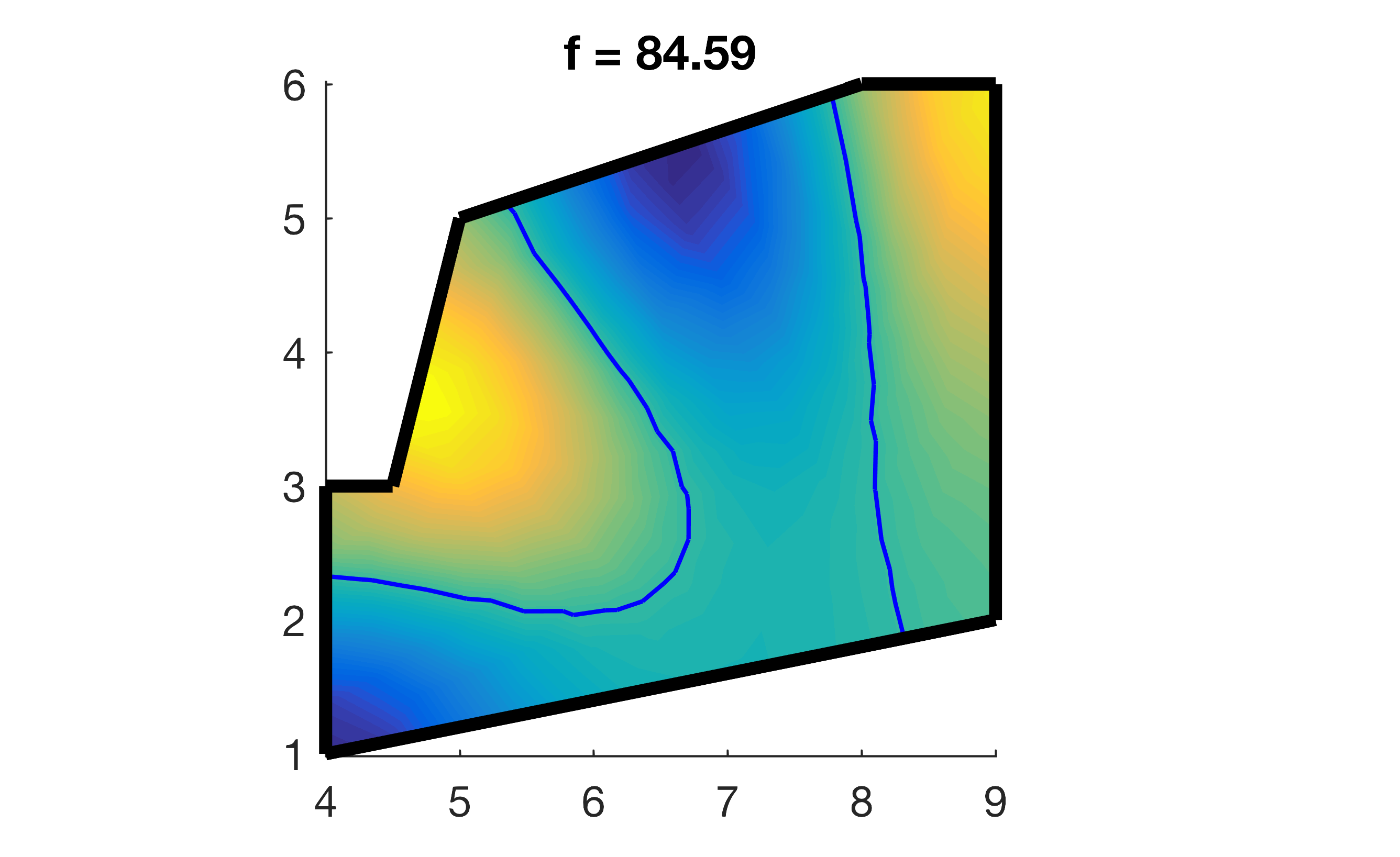
Some More Interesting Rooms

A similar bedroom, but perhaps with a 1m x 2.5m built in wardrobe along one edge, creating a small entry hallway.

Pressure eigenmodes of a room with a built in robe.

An oddly shaped polygonal room.

Pressure Eigenmodes of a polygonal room.

And the bedroom, connected to that polygonal room.

Pressure eigenmodes of two connected rooms.

You can see that the resonances of each individual room tend to remain somewhat independent (though slightly distorted), but new modes appear with as the rooms are coupled together.

Practical Impacts

Now that we can calculate the resonances, they may be used for a few things such as:

Inform room geometry at the design stage. Square/Rectangular rooms are typically undesirable for live/listening rooms (think about the predictable distribution of mode nodes/antinodes), but more complicated geometry has inherent unknowns. Eigenmode analysis can give valuable insights into a room’s frequency response before it is built.
Confirm frequency response of existing rooms. The frequency response of a room may reveal some problem resonances at selected frequencies, you may want to confirm they are from the room geometry.
Inform placement of acoustic treatment. You have a huge resonance, and you have a bass trap to try and kill it, but where should you place it? You want to avoid nodes, and place it at the antinodes, the spatial distribution can help with this.
Inform monitor placement. Speakers placed at nodal/antinodal points can be unpredictable (a resonance can’t be excited from a node, and is more easily excited from an antinode), knowing where they are can be extremely helpful.

You may have also noticed from the distribution plots that antinodes will frequently occur along boundaries, and in corners, which is why bass traps and treatment is usually placed there.

If you’re interested in the response of an atypical room, let me know the geometry and I can run the tool and post the results. Or if you have MATLAB and the PDE Toolbox, you can run the full script yourself, found below.

%EIGENMODEANALYSIS.m - Investigate acoustic eigenmodes of polygons.
%Searches for acoustic eigenmodes of a 2D polygonal geometry as specified
%by the user. Generate plots to visualise the spatial distribution, and
%store a vector of frequencies.
%
% User Variables:
%   polygonVerticies    - 2 x m matrix of x/y coordinates defining the
%                           polygonal geometry.
%   fRange              - [fMin fMax] vector defining the range to
%                           search for resonant frequencies (Hz).
%   medium_speed        - Speed of sound in the medium.
%
% Useful Outputs:
%   f       - Vector of calculated resonant frequencies in Hz.
%   model   - pde.PDEModel object containing the PDE information.
%   results - pde.EigenResults object with the results of the analysis.
%   h       - handle to figure object containing plots.
%
% Usage:
% Running the script with the below user paramters should give an idea
%   polygonVertices = [[0 1 1 0];[0 0 1 1]]; %[m]
%   fRange = [20 500]; %[Hz]
%   medium_speed = 343.0; % [m/s] 
%
%
% Author: Jonathan South
% JSouthAudio
% email: j.south@jsouthaudio.com
% Website: https://www.jsouthaudio.com
% August 2018; Last revision: 30-August-2018

%% User Setup

% x/y coordinates of the room geometry. Assumed closed polygon between last
% and first coords.
polygonVertices = [[0 1 1 0];[0 0 1 1 ]]; %[m]

% Interval to search for resonant frequencies
fRange = [20 500]; %[Hz]

% Wave speed of the medium on the region. Approx 343 m/s for air at STP.
medium_speed = 343.0; % [m/s]


%%%%%%%%%%%%%%%%%%%%%%%%%%%%%%%%%%%%%%%%%%%%%%%%%%%%%%%%%%%%%%%%%%%%%%%%%%%
%% Model Setup
disp('Setting up model...')
model = createpde();

% get the room geometry from the given vertices, and add it to model
model.geometryFromEdges(createRoomGeometry(polygonVertices(1,:), ...
    polygonVertices(2,:)));

% Coefficients for the eigenvalue problem. The pde tool solves in the form
% of - div(c*grad(u)) + a*u = lambda*d*u.
model.specifyCoefficients('m', 0, 'd', -(1/medium_speed).^2, 'c', -1,...
    'a', 0, 'f', 0);

% Apply the pressure boundary condition for a perfectly reflecting
% boundary. Neumann condition given in the form of n*(c*grad(u)) + q*u = g
model.applyBoundaryCondition('neumann', ...
    'Edge', 1:model.Geometry.NumEdges,'q',0, 'g',0);

% Mesh the domain.
model.generateMesh();

% Specify the Eigenvalue range. Corresponds to lambda = w^2
r = fRange*2*pi;
r = r.^2;

%% Solve
disp('Solving...')

% Solve the problem
results = model.solvepdeeig(r);

% extract the resonant frequencies. Eigenvalues are lambda = w^2, hence
f = sqrt(results.Eigenvalues)/(2*pi);

%% Visualise
disp('Generating Plots...')

h = visualiseEigenmodes(model, results);

disp('Done')

%%%%%%%%%%%%%%%%%%%%%%%%%%%%%%%%%%%%%%%%%%%%%%%%%%%%%%%%%%%%%%%%%%%%%%%%%%%
%% Helper Functions
function h = visualiseEigenmodes(model, results)
%VISUALISEEIGENMODES - Visualises spatial Eigenmodes from solvepdeeig
%Sometimes will generate an errant axis in the last position.
%
% Inputs:
%   model - pde.PDEModel object
%   results - pde.EigenResults object
%
% Outputs
%   h - handle to generated figure

% Get some values to layout the subplots nicely
nPlots = length(results.Eigenvalues);
spr = ceil(sqrt(nPlots));
spc = ceil(nPlots/spr);

% color for node lines on the plots
node_color = 'b';

h = figure;
h.set('Name', 'Spatial Eigenmode Distribution')

for n = 1:nPlots
    subplot(spr,spc,n); 
    % make the plot
    hp = pdeplot(model,'XYData', ...
        results.Eigenvectors(:,n)/max(abs(results.Eigenvectors(:,n))),...
        'Contour','on', 'Levels',[-1.1, 0, 1.1], 'Colormap', 'parula');
    axis equal    
    title(sprintf('f = %0.2f', sqrt(results.Eigenvalues(n))/(2*pi)));
    colorbar off

    % modify some visual aspects
    % change the nodal line weight
    node_lines = findobj(hp,'Type','line');
    for j = 1:length(node_lines)
        node_lines(j).set('LineWidth', 1.0, 'Color', node_color);
    end

    hold on
    % show the boundary
    hp = pdegplot(model);
    % change the boundary line weight
    boundary_lines = findobj(hp, 'Type', 'line');
    for j = 1:length(boundary_lines)
        boundary_lines(j).set('LineWidth', 3, 'Color', 'k');
    end

    % change axes bg color to transparent
    set(gca, 'Color', 'none');
end

% Set up the colorbar
% 'Position' Property is [left bottom width height]
first_plot = get(subplot(spr,spc, 1), 'Position');
last_plot = get(subplot(spr,spc, spr*spc), 'Position');

colorbar_position = [(last_plot(1)+last_plot(3))*1.1  ...
    last_plot(2)*1.1 ...
    last_plot(3)*0.10  ...
    ((first_plot(2)+first_plot(4))-last_plot(2))*0.9];
c= colorbar('Position', colorbar_position,...
    'Limits', [-1 1], 'Ticks', [-1, 0, 1], ...
    'TickLabels', {'-1 (Antinode)','0 (Node)', '1 (Antinode)'},...
'FontSize', 14);

c.Label.String = 'Relative Pressure Variation around Equilibrium';

% Set up a legend from the last node line
leg = legend([node_lines(end), boundary_lines(end)],...
    {'Pressure Nodes', 'Reflecting Boundary'});
leg_old_position = leg.get('Position');
leg_position = [0.5-leg_old_position(3)*0.5  ...
    1-leg_old_position(4) ...
    leg_old_position(3)  ...
    leg_old_position(4)];

set(legend, 'Position', leg_position, 'Units', 'normalized',...
    'FontSize', 14);
    
end

function dl = createRoomGeometry(x,y)
%CREATEROOMGEOMETRY - Generates polygon geometry for PDE from x/y vertices
%Polygon is assumed closed, by joining the last vertex to the first.
%Should not be self intersecting.
%
% Inputs:
%   x - 1 x m vector of polygon vertext x coordinates
%   y - 1 x m vector of polygon vertext y coordinates
%
% Outputs:
%
%   dl - Decomposed Geometry Matrix returned from PDE tool descg()

assert(length(x)==length(y), 'Vertex vectors are different lengths.');

% Setup the geometry vector as per required pdetool spec
gd(1) = 2;     % First row 2 for a polygon
gd(2) = length(x); % Second row number of boundary edges

% x values of vertices
gd(3:3+length(x)-1) =x;
% y values of vertices
gd(3+length(x):3+length(x)+length(y)-1) = y;
gd = gd';

% Output of csgchk is all zeros if it is valid geometry.
assert(sum(csgchk(gd))==0,...
    'Invalid Geometry. Potentially self-intersecting polygon.');

dl = decsg(gd);
end

Tags: acoustics, eigenmode, eigenvector, eignenvalue, frequency, helmholtz, matlab, model, pde, resonant, simulation